
The concept of statistical significance is central to planning, executing and evaluating A/B (and multivariate) tests, but at the same time it is the most misunderstood and misused statistical tool in internet marketing, conversion optimization, landing page optimization, and user testing. This is not my first take on the topic, but it is my best attempt to lay it out in as plain English as possible: covering every angle, but without going into math and unnecessary detail. The first part where I explain the concept is theory-heavy by necessity, while the second part is more practically-oriented, covering how to choose a proper statistical significance level, how to avoid common misinterpretations, misuses, etc.
What is statistical significance?
To explain it properly, we need to take a small step back to get the bigger picture, first. In many online marketing / UX activities, we aim to take actions that improve the business bottom-line: acquire more visitors, convert more visitors, generate higher revenue per visitor, increase retention and reduce churn, increase repeat orders, etc. However, knowing which actions lead to improvements is not a trivial task. This is where A/B testing comes into play, since an A/B test, a.k.a. online controlled experiment, is the only scientific way to establish a causal link between our (intended) action(s) and any results we observe. You can always choose to skip the science and go with your hunch, or to use just observational data. However, going the scientific way, you can estimate the effect of your involvement and basically predict the future (isn’t that the coolest thing!).
In an ideal world, we would be all-knowing and there would be no uncertainty, so experimentation will be unnecessary. However, in the real-world of online business, there are limitations we need to work with. In A/B testing we are limited by the time, resources and users we are happy to commit to any given test. What we do is we measure a sample of the potentially infinitely many future visitors to a site and then use our observations on that sample to predict how visitors would behave in the future. In any such measurement of a finite sample, in which we try to gain knowledge about a whole population and/or to make prediction about future behavior, there is inherent uncertainty in both our measurement and in our prediction.
This uncertainty is due to the natural variance of the behavior of the groups we observe. Its presence means that if we split our users into two randomly selected groups, we will observe noticeable differences between the behavior of these two groups, including on Key Performance Indicators such as e-commerce conversion rates, lead conversion rates, bounce rates, etc. Even without doing anything different to one group or the other, they will appear different. If you want to get a good idea of how this variance can play with your mind, just run a couple of A/A tests and observe the results over time. Most of the time you will notice distinctly different performance in the two groups, with the largest difference in the beginning and the smallest towards the end of however long you decide to run the test.
It is precisely this uncertainty, coupled with our desire to have a reliable prediction about the future, that necessitates the use of statistical significance, which is a tool for measuring the level of uncertainty in our data.
Statistical significance is useful in quantifying uncertainty.
But how does it help us quantify uncertainty? In order to use it, we design and execute a null-hypothesis statistical test[2], which is a case of Reductio ad absurdum argumentation. In such an argument, we examine what would have happened if something was true, until we reach a contradiction, which allows us to declare it false.
First, we chose a variable we want to measure our results by. Let’s use the difference in conversion rate for some action such as lead completion or purchase and let’s denote it by µ. Then, we define two statistical hypothesis, covering every possible value for µ that we might observe. Usually (but not always! See Non-inferiority testing below), one hypothesis (the null, or default hypothesis) is defined as our intervention having no positive effect, or having a negative effect (µ ≤ 0). The alternative hypothesis is that the changes we want to implement will have a positive effect (µ > 0).
In most tests, we know the probability of observing certain outcomes for any given true value, thus we have a simple mathematical model we can link to the real world. In an A/B test we examine the results and ask ourselves the following question: assuming the null hypothesis is true, how often, or how likely would it be that we’ll observe results that are as extreme or more extreme than the ones we observe. “Extreme” here just means “differing by a given amount”. This is precisely what statistical significance measures.
Statistical significance measures how likely it would be to observe what we observed, assuming the null hypothesis is true.
Here is a visual representation I’ve prepared, the example is with a commonly-used 95% threshold (one-sided p-value of 0.05):
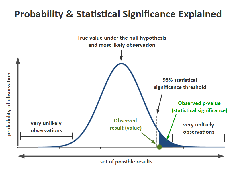
Statistical significance is then a proxy measure of the likelihood of committing the error of deciding that the statistical null hypothesis should be rejected, when in fact, we should have refrained from rejecting it. This is also referred to as a type I error, or an error of the first kind and a higher level of statistical significance means we have more guarantees against committing such an error.
Some of you might still be wondering: why would I want to know that, I just want to know if A is better than B, or vice versa?
What does it mean if a result is statistically significant*?
* at a given level
Logically, knowing that something is very unlikely to have occurred assuming the null hypothesis of no improvement, can mean that either one of these is true:
1.) There is a true improvement in the performance of our variant versus our control.
2.) There is no true improvement, but we happened to observe a rare outcome. The higher the statistical significance level, the rarer the event. For example, a 95% statistical significance would only be observed “by chance” 1 out of 20 times, assuming there is no improvement.
3.) The statistical model is invalid (does not reflect reality).
If you are measuring the difference in proportions, as in the difference between two conversion rates, you can dismiss #3 for all practical purposes since in this case the model is quite simple: classical binomial distribution, has few assumptions and is generally applicable to most situations. Still, there is a possibility that the distribution used is not suitable for analyzing our case. For example, don’t try to use binomial distribution to measure continuous outcomes such as revenue, as it will be a fairly clear case of the model not fitting reality. There are ways to test if the underlying distribution is of a given type, but this is a topic for a separate article.
So, knowing that a result is statistically significant with a p-value (measurement of statistical significance) of say 0.05, equivalent to 95% significance, you have a 1/20 chance that you would have observed what you observed due to natural variation. It is your measurement of uncertainty. If you are happy going forward with this much (or this little), uncertainty, then you have some quantifiable guarantees related to the effect and future performance of whatever you are testing.
The more technically inclined might consider this deeper take on the definition and interpretation of p-values.
It is probably as good a place as any to say that everything I state here about statistical significance and p-values is also valid for approaches relying on confidence intervals. Confidence intervals are based on exactly the same logic, so what is true for one, is true for the other. I usually recommend looking at both the p-value and a confidence interval to get a better understanding of the uncertainty surrounding your A/B test results.
Significance in non-inferiority A/B tests
While many online controlled experiments are designed as superiority tests, that is: the error of greater concern is that we will release a design, process, etc. that is not superior to the existing one, there is a good proportion of cases where this is not the error of primary concern. Instead, the error that we’d be trying to avoid most is that we fail to implement a non-inferior solution.
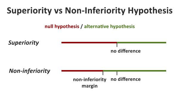
In these cases, the null hypothesis is defined as our intervention having a positive effect, or having a negative effect no larger than a given margin M: µ ≤ -M. The alternative hypothesis is that the changes we want to implement will have a positive effect or a negative effect smaller than M: µ > -M. M could be zero or positive. Naturally, in this case the interpretation of a statistically significant result will change: if we observe a statistically significant result the conclusion won’t be that there is true improvement of a given magnitude, but that the tested variant is just as good as our current solution, or better, and no worse than our chosen margin M.
To learn more on how to use such tests test to better align questions and statistics in A/B testing, and to speed up your tests, consult my comprehensive guide to non-inferiority AB tests.
Common misinterpretations of statistical significance
Falling prey to any of the below misinterpretations can lead to seriously bad decisions being made, so do your best to avoid them.
1. Treating low statistical significance as evidence (by itself) that there is no improvement
To illustrate it simply: let’s say you measure only 2 (two) users in each group for a given test and after doing the math your result is not statistically significant (has a very high p-value). Does it mean the data warrants you accept there is no improvement? Of course not, you would certainly say. Such an experiment doesn’t put this hypothesis through a severe test, that is: the test had literally zero chance to show a statistically significant result, even if there was a true difference of great magnitude. The same might be true with 200, 2,000 or even 200,000 users per arm, depending on the parameters of the test[3:2.5].
In order to reliably measure the uncertainty attached to a claim of no improvement, you need to look at the statistical power of the test. Statistical power measures the sensitivity of the test to a certain true effect, that is: how likely you would be to detect a real discrepancy of some minimum magnitude at a desired statistical significance level. (“Power analysis addresses the ability to reject the null hypothesis when it is false” (sic) [2])
If the power is high enough, and the result is not statistically significant, you can use reasoning similar to that of a statistically significant result and say: this test had 95% power to detect a 5% improvement at a 99% statistical significance threshold, if it truly existed, but it didn’t. That means we have good grounds to infer that the improvement, if any, is less than 5%.
2. Thinking high statistical significance equals substantive or practically relevant improvement
This is erroneous, since a statistically significant result can be so small in magnitude that it has no practical value. For example, a statistically significant improvement of 2% might not be worth implementing if the winner of the test will cost more to implement and maintain than what these 2% are worth in revenue over the next several years. The above is just an example, as what magnitude is practically relevant is subjective and the decision should be made on a case-by-case basis.

Some say this “failure” of statistical significance (it’s not a bug, it’s truly a feature!) is due to it being a directional measure only, but they’d be wrong[3:2.3]. A higher observed statistical significance (lower p-value) is evidence of a bigger magnitude of the effect, everything else being equal, so it is not directional only.
I agree though, that it might be hard to gauge how big of an effect one can reasonably expect by statistical significance alone. Therefore, it is a best practice to construct confidence intervals at one or several confidence levels, so you get a sense of the magnitude.
3. Treating statistical significance as the likelihood that the observed improvement is the actual improvement
Everything else equal, observing a higher statistical significance, is better evidence for a bigger true improvement than observing a lower one, however, it would be a significant error to directly attach the statistical significance measure to the observed result. Having such a certainty would usually require much, much more users or sessions. Here is a quick illustration:

While the observed lift is 20% and it has a high statistical significance, the 95% confidence interval shows that the true value for the lift is likely to be as low as 2.9% – blue numbers bellow % change are the confidence interval.
To get a measure of how big and how small a difference can be expected, it is best to examine the confidence intervals around the observed value. Maximum likelihood estimates also help in this regard.
4. Treating statistical significance as the likelihood that the alternative hypothesis is true or false
This is a common misconception, which gets especially bad if you mix it with misinterpretation #3 and you forget your alternative hypothesis is “A is better than control” and substitute it with “A is 20% better than control” (from the example above).
Attaching probabilities to any hypothesis that tries to explain the numbers is not something you can do using statistical significance or frequentist methods. Doing so would require an exhaustive list of hypotheses and prior probabilities, attached to them. This is the territory of Bayesian inference (inverse inference) and it is full of mines, so thread carefully, if you choose to explore it. If you are interested in my thoughts on the Bayesian “simplicity” temptation and other purported advantages of these approaches, read points #1 and #2 in “5 Reasons to go Bayesian in AB Testing: Debunked“.
Common mistakes in using statistical significance in A/B testing
Any of these mistakes will invalidate your statistical significance test, so take extra caution to avoid them by using proper tools and procedures, as the error can easily be multiples, not percentages of the expected one. What is common between them is that the nominal significance (or p-value, or z-value, or t-value) or confidence interval you will see, will not reflect the true rarity of what you observed, making the uncertainty measure useless or introducing significant and hard to measure bias. As the saying goes: Garbage In, Garbage Out.
1. Lack of fixed sample size or unaccounted peeking
This mistake happens when you are:
- using a simple significance test to evaluate data on a daily/weekly/etc. basis, stopping once you find a nominally statistically significant result. While it looks OK on the surface, most of the time it is not, since such simple tools require fixing your sample size in advance and only observing your data once – at the predetermined time/# of users. Do differently, and your uncertainty measure can be thrown off in the multiples. If this issue is not immediately obvious to you, I recommend a detailed discussion at “The bane of A/B testing: Reaching Statistical Significance“.
- fixing your sample size in advance, but peeking with the intent to stop either way
- using a proper sequential testing method, but failing to register your observations faithfully, so that the statistics can be adjusted accordingly
- using a Bayesian sequential testing method that claims immunity to optional stopping (why Bayesian approaches are not immune to optional stopping)
One way is to fix your sample size in advance and stick to just a single observation at the end of a test. It might be inflexible and inefficient, but you will know what is warranted by the data at hand. Alternatively, try a good sequential testing methodology, such as the AGILE A/B testing approach (our A/B testing calculator is available to make it easy for you to apply in your daily work). This way you gain flexibility and efficiency, with 20-80% faster tests.
2. Lack of adjustments for multiple testing
Multiple testing, also called multivariate testing or A/B/n testing, is when you test more than one variant against a control in a given test. This can lead to increased efficiency in some situations and is a fairly common practice, despite the drawback that it requires more time/users to run a test. Analyzing such a test by either picking the best variant and doing a t-test / z-test / chi-square test, etc. on the control and that variant, or doing one such test for each variant against the control significantly increases the Family-Wise Error Rate (FWER) since there are more hypothesis being tested, thus we increase the chance of getting a false positive.
There are special procedures for accounting for it with Dunnett’s post-hoc adjustment being the preferred method. It is also the one used in AGILE A/B testing. For more, read our detailed guide to multivariate testing in which I discuss when is such a test more efficient, among other things.
3. Lack of adjustments for multiple comparisons
Multiple comparisons happen when you have more than one endpoint for a test and it is another example of increasing the Family-Wise Error Rate. For example, you take into account (and hopefully do statistical analysis on): bounce rate differences, add to cart conversion rate differences, purchase completion conversion rate differences, all in one test. Doing more than one comparison between the groups makes it more likely that one of them will turn out statistically significant. There are different procedures for this scenario, but I believe the classical Bonferroni correction should be the preferred one. We’ve also examined Benjamini-Hofberg-Yekutieli’s false discovery rate procedures, but found them inappropriate for the typical A/B testing scenario.
Bonus mistake: using two-tailed tests and interpreting them as one-tailed tests. This is very common, especially since a lot of vendors seem to be using and reporting two-sided significance. I’ve written a whole separate article on this here: one-tailed vs. two-tailed significance tests in A/B testing.
How to choose an appropriate statistical significance level?
Many people have issues when it comes time to choose the statistical significance level they want and it is due to a simple fact: there are trade-offs involved. The major trade-offs are between speed, flexibility and efficiency on one side, and accuracy, certainty, sensitivity and predictability on another.
The major trade-offs in A/B testing are between speed, flexibility and efficiency on one side, and accuracy, certainty, sensitivity and predictability on another.
No matter what kind of statistical method you are using, you will end up with the following trade-offs:
- increasing the required statistical significance threshold means increasing the required sample size, thus slower testing;
- increasing the certainty about the true difference, equivalent to decreasing the width of the confidence interval, means increasing the required sample size, thus slower testing;
- increasing the statistical power (test sensitivity to true effects) means increasing the required sample size, thus slower testing;
- decreasing the minimum detectable effect size means (with a given power and significance) means increasing the required sample size, thus slower testing;
- increasing the sample size (time to run a test) means better certainty and/or higher test sensitivity and/or the same sensitivity towards a smaller effect size.
Several questions emerge quickly even from the brief summary above. Questions like: Shall I test longer, for better certainty, or should I test faster, accepting more frequent failures? Should I run quick, under-powered tests, seeking improvements of significant magnitude while missing smaller opportunities? Unfortunately, there are no easy answers in A/B testing methodology about what values you should choose for the main parameters of a statistical test.
Contrary to popular belief, the answers don’t get easier if you have more users and sessions at your disposal (huge, high-trafficked site), nor do they become especially harder with small sites that barely get any traffic and conversions.
That is because while high-trafficked and high-converting sites have more users to run tests on, it usually also means that even the slightest improvements can result in many thousands or even millions of dollars worth of revenue or profits. This warrants running highly sensitive tests, and high power quickly ramps up the user requirements to levels where even the most visited sites on earth need weeks or months to run a proper test. Making even small errors is equally costly, pushing statistical significance requirements higher, and thus slowing down testing even further.
Conversely, having few visits and conversions means that you must aim for big improvements in whatever you do, if A/B testing is even going to be worth it. On the other hand, if you are small AND nimble, you can accept higher uncertainty in what you implement, or be able to test so fast, that the lower sensitivity is not such a great issue.
My advice is to weigh the costs for designing, preparing and running the A/B test against the potential benefits (with a reasonable future extrapolation, e.g. several years) and see the sample sizes (and thus time) required by several different combinations of values for the three main parameters (significance, power, minimum effect size). Then, chose a statistical design that hits closest to the perfect balance. Using a flexible sequential testing framework such as AGILE can make the decision on the minimum effect size much easier, since in case the true difference is much larger or much smaller, the test will simply stop early so the efficiency sacrificed will be minimal.
There are some good practices that should be followed irrespective of what the sample sizes allow. For example, analyzing (sequential) tests on a weekly basis and not running tests for less than a week. For many businesses Tuesdays are not the same as Sundays, and even if you can run a satisfactory test in 3 days, you better plan it for a full seven days. Other best-practice advice can be found in white papers and books written by experts in the field.
While I don’t think there is a recipe for a perfect A/B test, I think the above advice for making a choice while facing several trade-offs is a helpful starting point for CRO and UX practitioners.
(Added Apr 27, 2018): I have subsequently developed a comprehensive overview of the costs & benefits and risks & rewards in A/B testing and have built a tool that will do the balancing act for you, allowing you to use A/B testing to manage business risk while maximizing gains and rewards: the A/B Testing ROI Calculator.
Closing thoughts
While statistical significance testing is a powerful tool in the arms of a good CRO or UX expert, it is not a panacea or substitute for expertise, for well-researched and well-designed tests. It is a fairly complex concept to grasp, apply appropriately, and communicate to uninformed clients. I hope this post, which is a natural continuation of years of work on A/B testing statistical theory and methodology, helps shed light and can be a handy guide for the uninitiated.
References:
[1] Aberson, C. L. (2010) – “Applied Power Analysis for the Behavioral Sciences”, New York, NY, Routledge Taylor & Francis Group
[2] Fisher, R.A. (1935) – “The Design of Experiments”, Edinburgh: Oliver & Boyd
[3] Mayo, D.G., Spanos, A. (2010) – “Error Statistics”, in P. S. Bandyopadhyay & M. R. Forster (Eds.), Philosophy of Statistics, (7, 152–198). Handbook of the Philosophy of Science. The Netherlands: Elsevier.